Friday, June 27, 2008

A4-Enhancement by Histogram Manipulation

The goal is to improve the quality of a grayscale image by manipulating its histogram. One method is by modifying the image's PDF(Probability Distribution Function) using its CDF(Cumulative Distribution Function).
I will try to improve the quality of the image below:

Figure 1: photo.jpg

Figure 2: Histogram of photo.jpg using ImageJ

It can be observed from the two figures that the image's quality is poor since a large number of pixels accumulate in a small range of the grayscale values. The image's information are as follows:

FileName: friends.jpg
FileSize: 2865

Format: JPEG

Width: 164

Height: 194

Depth: 8

StorageType: indexed

NumberOfColors: 256
ResolutionUnit: inch
XResolution: 72.000000

YResolution: 72.000000


I. In a separate scipad, I defined the following functions and save it as "myfunc.sce":

-->function [X,Y,L,V,W,Z]=myfunctions(im);
-->X=[];

-->Y=[];
-->L=[];
-->v=1;
-->for i=0:1:255;
-->[x,y]=find(im==i);

-->X(v)=i; // gives the grayscale value
-->Y(v)=length(x); //gives the number of pixels
-->L(v)=(v-128)./255; // this is for the function that will give a theoretical CDF
-->v=v+1;

-->end;
-->V=(0.5.*tanh(5.*L))+1; // Function of the theoretical CDF I wish to obtain later
-->W=Y/c; // normalizes Y
-->Z=cumsum(W); //gives the normalized cumulative sum of Y
-->endfunction;

II. Now, in Scilab's command window:

-->im=imread('photo.jpg');// loads the image in Scilab
-->a=size(im,1);
-->b=size(im,2);
-->c=a.*b; //gives the total size of the image
-->getf('myfunc.sce'); //gets the function from the file "myfunc.sce" -->[X,Y,L,V,W,Z]=myfunctions(im); // Loads the functions in I

To plot the histogram:

-->plot(X,Y); //plots the histogram

Figure 3: Histogram of photo.jpg

To plot the PDF/normalized histogram:

-->xbasc(); // clears the previous plot in the graphics window
-->plot(X,W);
Figure 4: PDF of photo.jpg

To plot the CDF:

-->xbasc();
-->plot(X,Z); //plots the CDF

Figure 5:CDF of photo.jpg

To plot the theoretical CDF:

-->xbasc();
-->plot(X,V); //plots the the theoretical CDF

Figure 6: Theoretical CDF

To enhance the image's quality, I replaced each pixel value by the image's CDF value.

-->photo1=[];
-->for e=1:1:a;
-->for f=1:1:b;
-->photo1(e,f)=Z(im(e,f));
-->end;
-->end;
-->imwrite(photo1,'photo1.jpg');

Here is the new image:
Figure 7: photo1.jpg

III. In a new scilab window, I simply repeated step II and change 'photo.jpg' to 'photo1.jpg' and here are the results:

Figure 8:Histogram of photo1.jpg

Figure 9: PDF of photo1.jpg

Figure 10: CDF photo1.jpg

IV. I tried producing a non-linear CDF that will mimic the CD of the human eye. For this part, the function "V=(0.5.*tanh(5.*L))+1" in Step I will serve as the theoretical CDF. I first used the CDF of 'photo.jpg.' For each grayscale value on the x-axis, I need to obtain its corresponding value on the y-axis (See Figure 5). I will then substitute this with the values of theoretical CDF (i.e V, see Figure 6). By taking the inverse of V, a new set of grayscale values were obtained. The result is a new image with a wider range of grayscale values, and hence a better contrast. The codes are written below:

-->im=imread('photo.jpg');
-->a=size(im,1);
-->b=size(im,2);
-->c=a.*b;
-->getf('myfunc.sce');
-->[X,Y,L,V,W,Z]=myfunctions(im);
-->w=[0:255]; // new set of gray scale values
-->//To get the projection of the grayscale value of the untreated image on its CDF I used
-->A=interp1(X,Z,im);
-->//To replace the projection above with the theoretical CDF and project this on a new grayscale value I used
-->B=interp1(V,w,A);
-->C=B./255;
-->imwrite(C,'photo2.jpg');

The resulting image is as follows:
Figure 11: photo2.jpg

V. By repeating step II and substituting 'photo.jpg' by 'photo2.jpg', the plots for the image are below:

Figure 12:Histogram of photo2.jpg


Figure 13: PDF of photo2.jpg

Figure 14: CDF of photo2.jpg

In last two images, the contrast of the image improved because image pixels can be found in all grayscale values. It can also be observed that the last two photos lack "smoothness" in comparison to the original photo. I think that this is due to the peaks found in their histograms. The variation in the length of the peaks causes the non-continuity of the grayscale values in each pixel. But as of the moment, I still can't figure out how to arrange this.

I rate myself 10/10 for this activity.


Photo Source:

http://www.american-indian-artwork.com/restoration/grayscale-picture-650.jpg

Wednesday, June 25, 2008

A3-Image Types and Basic Image Enhancement

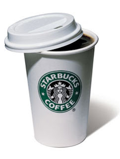
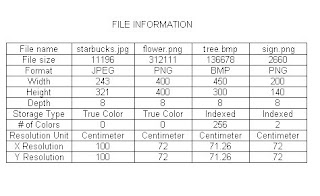
In this activity, scilab was used to display the different properties of the images available.filename: starbucks.jpg

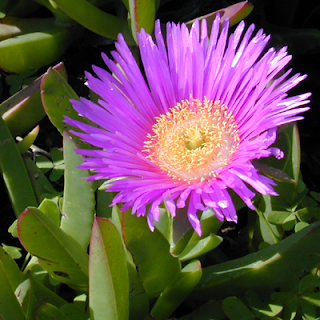
filename: flower.png


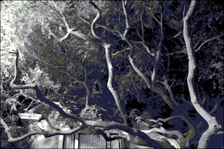
filename: tree.bmp

filename: sign.png


The images above were saved in the computer with their corresponding file names. Here is how to display the image's property:
  • The first image was saved using the file name "starbucks.jpg"
  • The following codes were then typed into scilab

--> starbucks = imread('starbucks.png'); // This will read the image into scilab
--> info = imfinfo('starbucks.png','verbose');

  • The following information will be then displayed:

File Name: starbucks.jpg
File Size : 11196
Format: JPEG
Width: 243
Height: 321
Depth: 8
Storage Type: True Color
Number of Colors: 0
Resolution Unit: Centimeter
X Resolution: 100
Y Resolution: 100


By doing the same method to the other images, the following information were collected:

For this activity, the goal was to obtain the area of a scanned flat object using Scilab. To do this, a process called thresholding was used. This process allows image segmentation or it converts a grayscale image to a binary image. I chose a 100 peso bill as my object and its scanned image appears below.

money.jpg

The step by step process is written below with the "-->" preceding each codes that was used.

1. Usually, a scanned image has a large memory hence I first increased the stack size to 20MB.

-->stacksize(20000000);

2. Using the same method that appears above, I loaded the file money.jpg into scilab and display its information

-->Img=imread('money.jpg');

-->Info1=imfinfo('money.jpg','verbose');

The following information will then be displayed:

FileName: money.jpg

FileSize: 148722

Format: JPEG

Width: 960

Height: 416

Depth: 8

StorageType: truecolor

NumberOfColors: 0

ResolutionUnit: inch

XResolution: 150.000000

YResolution: 150.000000

3. I then converted this to grayscale image:

-->Img=Img(:,:,1);

-->imwrite(Img(:,:),'money1.jpg');

-->Img=imread('money1.jpg');

-->Info2=imfinfo('money1.jpg','verbose');

FileName: money1.jpg

FileSize: 126567

Format: JPEG

Width: 960

Height: 416

Depth: 8

StorageType: indexed

NumberOfColors: 256

ResolutionUnit: inch

XResolution: 72.000000

YResolution: 72.000000

money1.jpg

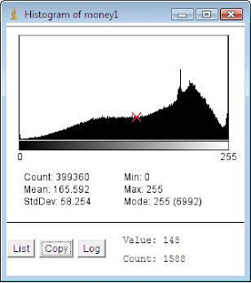
4. To do thresholding,I first obtained a histogram of money1.jpg. There are two ways to obtain a histogram. One way open this in ImageJ, which gives the histogram that appears below.

Scilab can also display a histogram of the same image using the following codes:

-->gs_val=[]

-->pixel_num=[]

-->counter=1;

-->for i=0:1:255

-->[x,y]=find(Img==i);

-->gs_val(counter)=i;

-->pixel_num(counter)=length(x);

-->counter = counter+1;

-->end;

-->plot(gs_val,pixel_num);


The y axis is the number of pixels and the x axis is the grayscale value. From the histogram, it can be observed that the image has a good contrast since all the grayscale values are occupied. The red mark on both images is the threshold value which is 148. This value will determine if a pixel will be given a value of "0" or "1".

5. Using the following.

-->BW=im2bw(Img, 0.580);

-->BS=abs(BW-1);

-->imshow(BS);

The result is the binary image below.

money3.bmp

The information is as follows.

FileName: Untitled.bmp
FileSize: 26286
Format: BMP
Width: 673
Height: 298
Depth: 8
StorageType: indexed
NumberOfColors: 2
ResolutionUnit: centimeter
XResolution: 0.000000
YResolution: 0.000000

5. Finally, we apply the area calculation in A2 blog.

-->[w,z]=follow(BW) //to obtain the edge pixel values of the image

-->X=size(w,1); //this gives the width of the image

-->Y=size(z,1); // this gives the height of the image

-->w2(1)=w(X);

-->w2(2:X)=w(1:X-1); // this was used for iteration

-->z2(1)=z(Y);

-->z2(2:Y)=z(1:Y-1);

-->A = 0.5.*sum(w.*z2-z.*w2);

-->Area=abs(A)

Scilab gave an area of 397985 and the actual area of the image is 360384 (932X387). The error was computed to be 10.3%.


In Windows, the image's properties are as follows:

This can be seen by right clicking the image, click on Properties > Details.

Thursday, June 19, 2008

Area Estimation of Images with defined Edges

The exercise was to compute the area of the square above with dimensions of 100*100. The filename saved is "square.bmp"

Green's theorem was used to obtain a formula for the area of an image in grayscale

The codes for the area estimation is as follows:

Image=imread('square.bmp') // to load the image in scilab
xbasc()
imshow(Image)
[x,y]=follow(Image) //to obtain the edge pixel values of the image
X=size(x,1); //this gives the width of the image
Y=size(y,1); // this gives the height of the image
x2(1)=x(X);
x2(2:X)=x(1:X-1); // this was used for iteration
y2(1)=y(X);
y2(2:X)=y(1:X-1);

Area = 0.5.*sum(x.*y2-y.*x2)

and this gives me an area of 9216 with a percent error of 7.84%

Beth and Rica helped me in this exercise ;)

I rate myself 10/10 for this exercise

Wednesday, June 11, 2008

A1-Digital Scanning


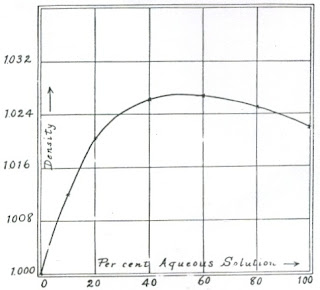
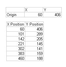
How I made the graph

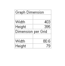
1. The total dimension was measured using the Create a Line button in the Tool Box.

2. The obtained dimension was divided by the number of data points in the X- and Y-axis.
3. Using the mouse pointer, the location of the origin and of the data points were determined.
4. The origin was subtracted from each data point position.

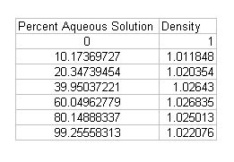
5. Using the following formula, the physical value of each data points were obtained.

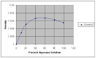
6. Using the Chart options, the obtained data were plotted.

I rate myself 9 out of 10 for the effort in this activity.