A3-Image Types and Basic Image Enhancement

In this activity, scilab was used to display the different properties of the images available.filename: starbucks.jpg

filename: flower.png

filename: tree.bmp

filename: sign.png

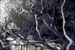
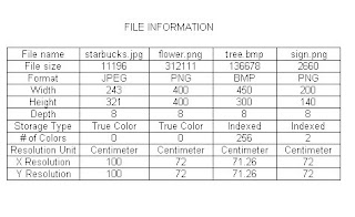
The images above were saved in the computer with their corresponding file names. Here is how to display the image's property:

• The first image was saved using the file name "starbucks.jpg"
• The following codes were then typed into scilab

--> starbucks = imread('starbucks.png'); // This will read the image into scilab
--> info = imfinfo('starbucks.png','verbose');

• The following information will be then displayed:

File Name: starbucks.jpg
File Size : 11196
Format: JPEG
Width: 243
Height: 321
Depth: 8
Storage Type: True Color
Number of Colors: 0
Resolution Unit: Centimeter
X Resolution: 100
Y Resolution: 100


By doing the same method to the other images, the following information were collected:

For this activity, the goal was to obtain the area of a scanned flat object using Scilab. To do this, a process called thresholding was used. This process allows image segmentation or it converts a grayscale image to a binary image. I chose a 100 peso bill as my object and its scanned image appears below.

money.jpg

The step by step process is written below with the "-->" preceding each codes that was used.

1. Usually, a scanned image has a large memory hence I first increased the stack size to 20MB.

-->stacksize(20000000);

2. Using the same method that appears above, I loaded the file money.jpg into scilab and display its information

-->Img=imread('money.jpg');

-->Info1=imfinfo('money.jpg','verbose');

The following information will then be displayed:

FileName: money.jpg

FileSize: 148722

Format: JPEG

Width: 960

Height: 416

Depth: 8

StorageType: truecolor

NumberOfColors: 0

ResolutionUnit: inch

XResolution: 150.000000

YResolution: 150.000000

3. I then converted this to grayscale image:

-->Img=Img(:,:,1);

-->imwrite(Img(:,:),'money1.jpg');

-->Img=imread('money1.jpg');

-->Info2=imfinfo('money1.jpg','verbose');

FileName: money1.jpg

FileSize: 126567

Format: JPEG

Width: 960

Height: 416

Depth: 8

StorageType: indexed

NumberOfColors: 256

ResolutionUnit: inch

XResolution: 72.000000

YResolution: 72.000000

money1.jpg

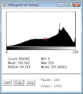
4. To do thresholding,I first obtained a histogram of money1.jpg. There are two ways to obtain a histogram. One way open this in ImageJ, which gives the histogram that appears below.

Scilab can also display a histogram of the same image using the following codes:

-->gs_val=[]

-->pixel_num=[]

-->counter=1;

-->for i=0:1:255

-->[x,y]=find(Img==i);

-->gs_val(counter)=i;

-->pixel_num(counter)=length(x);

-->counter = counter+1;

-->end;

-->plot(gs_val,pixel_num);

The y axis is the number of pixels and the x axis is the grayscale value. From the histogram, it can be observed that the image has a good contrast since all the grayscale values are occupied. The red mark on both images is the threshold value which is 148. This value will determine if a pixel will be given a value of "0" or "1".

5. Using the following.

-->BW=im2bw(Img, 0.580);

-->BS=abs(BW-1);

-->imshow(BS);

The result is the binary image below.

money3.bmp

The information is as follows.

FileName: Untitled.bmp
FileSize: 26286
Format: BMP
Width: 673
Height: 298
Depth: 8
StorageType: indexed
NumberOfColors: 2
ResolutionUnit: centimeter
XResolution: 0.000000
YResolution: 0.000000

5. Finally, we apply the area calculation in A2 blog.

-->[w,z]=follow(BW) //to obtain the edge pixel values of the image

-->X=size(w,1); //this gives the width of the image

-->Y=size(z,1); // this gives the height of the image

-->w2(1)=w(X);

-->w2(2:X)=w(1:X-1); // this was used for iteration

-->z2(1)=z(Y);

-->z2(2:Y)=z(1:Y-1);

-->A = 0.5.*sum(w.*z2-z.*w2);

-->Area=abs(A)

Scilab gave an area of 397985 and the actual area of the image is 360384 (932X387). The error was computed to be 10.3%.

In Windows, the image's properties are as follows:

This can be seen by right clicking the image, click on Properties > Details.